Talking Tokens

Ever wondered how AI, from creating images to writing text, actually “thinks”? It’s not a monolithic brain, but rather an intricate network built from countless tiny components. To truly grasp AI’s capabilities, we need to understand its fundamental building blocks: tokens.

Think of the human brain. Its astounding ability to process information and generate thoughts comes from billions of individual brain cells, or neurons, each connecting and firing signals in complex patterns.

In much the same way, if an entire AI model is like the vast human brain, then AI tokens are its individual brain cells.

WHY

The answer lies in the fundamental nature of how computers process information, it only understands numbers.

HOW

AI doesn’t just “read” text; it breaks it down into tokens using a tokenizer. Think of a tokenizer as a linguistic surgeon, dissecting raw text into meaningful units.

The exact method varies, but the general process is:

Break Down Text: The tokenizer first splits continuous text into smaller units. This isn’t just splitting by spaces. There are different types of splitting stratgegies used, below table summarizes the pros and cons of each, and looking at it you can guess why the most popular one is Subword tokenization

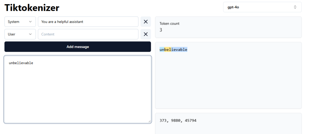
Subword tokenization (like BPE or WordPiece) is common for large language models. It smartly balances word and character-level approaches. It identifies common characters and sequences, then merges frequent pairs into new, longer subwords. This allows the AI to understand both common words and rare ones by breaking them into familiar subword units (e.g., “unbelievable” becomes [“un”, “believe”, “able”]).

Assign Numerical IDs: Each unique token is then given a unique numerical ID. This ID is the AI’s actual language (e.g., “the” becomes 123).

Great way to visualize the token generation is to use tiktok, just kidding, its to use tiktokenizer

If you simply type the word “unbelievable” you can see how one word generates 3 or more tokens.

Tokenization is a crucial step, but it’s part of a much longer journey. Significant processes, starting with data gathering and continuing well beyond tokenization, are necessary before we arrive at a sophisticated LLM like ChatGPT. This intricate pipeline owes much to the insightful, freely available content from Andrej Karpathy on YouTube. More to come.

Now, go fix some bugs!

Splitting Up Without Breaking Up: Partitioning Your Database with Style

WHY

In the high-stakes world of database management, sometimes the healthiest relationship is one with boundaries. If your database is starting to feel overwhelmed, sluggish, or just plain unmanageable, it might be time for the “we need to talk” conversation. But don’t worry—this isn’t a breakup; it’s a strategic restructuring that will make your relationship with your data stronger.

WHAT

Think of partitioning as sharding’s more localized cousin — a way to break up data within a single database or server to improve performance, maintainability, and query efficiency. While sharding is about splitting data across multiple nodes, partitioning is about organizing data smarter within the same node. Database partitioning is the practice of dividing a database table into smaller, more manageable segments based on defined rules while maintaining the logical appearance of a single table to applications interacting with it.

ANALOGY

Database partitioning is like organizing a clothing store where instead of piling all merchandise (data) into one massive, chaotic section, you thoughtfully arrange men’s, women’s, and children’s clothes into separate departments (partitions). Shoppers can easily find what they need, store employees can efficiently manage inventory and restocking for their specific section, and the store can expand by adding specialized sections without disrupting the existing layout – all while maintaining a seamless shopping experience.

HOW

Just as there are multiple ways to organize a closet, databases offer several partitioning strategies, each with its own strengths:

  • Horizontal Partitioning (Row-Based):Splits table rows across partitions based on ranges of a column value, like dividing customer records by date ranges or ID ranges.
  • Vertical Partitioning (Column-Based): Separates columns of a table into different partitions, typically grouping frequently accessed columns together and rarely used columns in separate partitions.
  • Functional Partitioning: Organizes data based on how it’s used in your application, grouping related tables or functionality together regardless of structural similarities.
  • List Partitioning: Divides data based on specific, discrete values in a column, such as storing customer data in different partitions based on country or region.
  • Hash Partitioning: Distributes rows evenly across partitions using a hash function on the partition key, ideal when natural groupings don’t exist or balanced distribution is critical.
  • Composite Partitioning: Combines multiple partitioning strategies, such as first partitioning by date range, then sub-partitioning each range by region or customer type.

Let’s look at an example with range partitioning the most common one

Let’s say you have a table called orders, and you want to partition it by order_date, one partition per year.

1. Create the Partitioned Table

CREATE TABLE orders (
    id SERIAL PRIMARY KEY,
    customer_id INT NOT NULL,
    order_date DATE NOT NULL,
    amount NUMERIC
) PARTITION BY RANGE (order_date);

2. Create Yearly Partitions

CREATE TABLE orders_2023 PARTITION OF orders
    FOR VALUES FROM ('2023-01-01') TO ('2024-01-01');

CREATE TABLE orders_2024 PARTITION OF orders
    FOR VALUES FROM ('2024-01-01') TO ('2025-01-01');

CREATE TABLE orders_2025 PARTITION OF orders
    FOR VALUES FROM ('2025-01-01') TO ('2026-01-01');

3. Insert Data (Postgres Routes Automatically)

INSERT INTO orders (customer_id, order_date, amount)
VALUES 
    (101, '2023-03-15', 200.00),
    (102, '2024-07-01', 350.00),
    (103, '2025-01-20', 500.00);

4. Query Normally

SELECT * FROM orders WHERE order_date >= '2024-01-01';

PostgreSQL will automatically prune irrelevant partitions during the query for performance gains.

Now, go fix some bugs!

Sharding is Caring: Distributing the Load for Database Health

Definition of the word

shard /ʃɑːd/ noun

a piece of broken ceramic, metal, glass, or rock, typically having sharp edges.”shards of glass flew in all directions”

Why

In today’s data-driven world, success often means rapid growth – and with that growth comes increasingly massive datasets. Traditional database setups eventually hit performance walls: queries slow down, hardware costs skyrocket, and your once-nimble application becomes sluggish under the weight of its own data.

Analogy

The Single Database Way (One Platform):
Imagine you have just one train platform at a busy station. Every train — whether it’s going north, south, east, or west — has to use that same platform. Passengers have to wait while a train arrives, unloads, loads, and departs before the next train can come in. It gets crowded fast, delays pile up, and the station staff struggles to manage the constant flow.

The Sharding Way (Multiple Platforms):
Now imagine you build separate platforms for different train lines — one for northbound trains, one for southbound, another for eastbound, and so on. Passengers go directly to the platform for their route, trains arrive and depart simultaneously on different tracks, and everything runs much more smoothly. The workload is divided, delays are reduced, and the station is far more efficient.

How

Database sharding offers a strategic solution by horizontally partitioning your data across multiple separate database instances. Rather than scaling up a single monolithic database (expensive and eventually impossible), sharding lets you scale out by distributing the load across multiple machines.

1. Application-Level Sharding (Manual)

  • How it works: Your app logic decides which database to write/read from based on a sharding key (e.g., user ID).
  • Pros:
    • Simple and flexible.
    • Works with vanilla PostgreSQL.
  • Cons:
    • App becomes tightly coupled to shard logic.
    • Cross-shard queries are hard to manage.

Use case: SaaS apps with clean tenant separation.


2. Foreign Data Wrappers (FDW)

  • Use postgres_fdw to link multiple Postgres servers and query them as if they’re one.
  • Each shard is a separate PostgreSQL instance, and a coordinator node aggregates results.
  • Pros:
    • Works with standard Postgres.
    • Allows federated queries.
  • Cons:
    • Limited optimizer support.
    • Performance penalty for cross-shard joins.

3. Citus (PostgreSQL Extension)

  • Distributed PostgreSQL: Citus transforms Postgres into a horizontally scalable database.
  • Supports real-time distributed SQL queries.
  • Handles sharding, replication, and distributed transactions.
  • Pros:
    • Automatic sharding and parallelism.
    • Supports complex queries and joins.
  • Cons:
    • Requires Citus installation.
    • Some Postgres features may be limited.

Use case: Real-time analytics, multi-tenant apps.

4. Schema-Based Sharding

  • Create multiple schemas in one Postgres instance, each acting like a shard.
  • Good for multi-tenant apps where each tenant gets a schema.
  • Pros:
    • Simple to manage.
    • No extra tooling.
  • Cons:
    • Doesn’t scale across machines.
    • Can hit performance limits at scale.

5. Hash-Based or Range-Based Sharding (Custom)

  • Partition data based on a hash or range of a sharding key (like user_id) and route queries accordingly.
  • Can be implemented with:
    • Partitioned tables (Postgres 10+).
    • Application logic or proxy routing.
  • Pros:
    • Better distribution control.
  • Cons:
    • Requires custom coordination and routing logic.

6. Proxy-Based Sharding

  • Use a proxy layer (like Pgpool-II, Odyssey, or custom reverse proxies) to manage routing and connections to shards.
  • Can perform load balancing and failover too.
  • Cons:
    • Adds latency and complexity.
    • Doesn’t inherently solve cross-shard consistency.

Simple Example implementation with EF

using Microsoft.EntityFrameworkCore;
using Microsoft.Extensions.DependencyInjection;
using System;
using System.Collections.Generic;
using System.Linq;
using System.Threading.Tasks;

public class Customer
{
    public int Id { get; set; }
    public string Name { get; set; }
    public string Email { get; set; }
    public DateTime CreatedAt { get; set; }
}

public class ShardDbContext : DbContext
{
    public ShardDbContext(DbContextOptions options) : base(options)
    {
    }

    public DbSet<Customer> Customers { get; set; }

    protected override void OnModelCreating(ModelBuilder modelBuilder)
    {
        modelBuilder.Entity<Customer>()
            .HasKey(c => c.Id);
    }
}

public class ShardingManager
{
    private readonly Dictionary<int, string> _shardMap = new Dictionary<int, string>
    {

        { 1, "Server=shard1.example.com;Database=Tenant1Db;User Id=user;Password=password;" },
        { 2, "Server=shard2.example.com;Database=Tenant2Db;User Id=user;Password=password;" },
        { 3, "Server=shard3.example.com;Database=Tenant3Db;User Id=user;Password=password;" }
    };

    public string GetConnectionString(int tenantId)
    {
        if (_shardMap.TryGetValue(tenantId, out string connectionString))
        {
            return connectionString;
        }
        
        throw new KeyNotFoundException($"No shard configured for tenant {tenantId}");
    }
}

public class ShardDbContextFactory
{
    private readonly ShardingManager _shardingManager;
    
    public ShardDbContextFactory(ShardingManager shardingManager)
    {
        _shardingManager = shardingManager;
    }
    
    public ShardDbContext CreateDbContext(int tenantId)
    {
        var connectionString = _shardingManager.GetConnectionString(tenantId);
        
        var optionsBuilder = new DbContextOptionsBuilder<ShardDbContext>();
        optionsBuilder.UseNpgsql(connectionString);
        
        return new ShardDbContext(optionsBuilder.Options);
    }
}

public class CustomerRepository
{
    private readonly ShardDbContextFactory _contextFactory;
    
    public CustomerRepository(ShardDbContextFactory contextFactory)
    {
        _contextFactory = contextFactory;
    }
    
    public async Task<Customer> GetCustomerAsync(int tenantId, int customerId)
    {
        using var dbContext = _contextFactory.CreateDbContext(tenantId);
        return await dbContext.Customers.FindAsync(customerId);
    }
    
    public async Task<List<Customer>> GetAllCustomersAsync(int tenantId)
    {
        using var dbContext = _contextFactory.CreateDbContext(tenantId);
        return await dbContext.Customers.ToListAsync();
    }
    
    public async Task AddCustomerAsync(int tenantId, Customer customer)
    {
        using var dbContext = _contextFactory.CreateDbContext(tenantId);
        dbContext.Customers.Add(customer);
        await dbContext.SaveChangesAsync();
    }
    
    public async Task<List<Customer>> GetCustomersFromAllShards()
    {
        var allCustomers = new List<Customer>();
  
        foreach (var tenantId in new[] { 1, 2, 3 }) // Hardcoded for simplicity
        {
            using var dbContext = _contextFactory.CreateDbContext(tenantId);
            var customers = await dbContext.Customers.ToListAsync();
            allCustomers.AddRange(customers);
        }
        
        return allCustomers;
    }
}

public class Program
{
    public static void Main(string[] args)
    {
        var services = new ServiceCollection();        
        services.AddSingleton<ShardingManager>();
        services.AddSingleton<ShardDbContextFactory>();
        services.AddScoped<CustomerRepository>();
        
        var serviceProvider = services.BuildServiceProvider();
      
        var customerRepo = serviceProvider.GetRequiredService<CustomerRepository>();
      
        ExampleUsageAsync(customerRepo).Wait();
    }
    
    private static async Task ExampleUsageAsync(CustomerRepository repository)
    {
        int currentTenantId = 1;
        
        await repository.AddCustomerAsync(currentTenantId, new Customer
        {
            Name = "John Doe",
            Email = "john@example.com",
            CreatedAt = DateTime.UtcNow
        });
        
        var customers = await repository.GetAllCustomersAsync(currentTenantId);
        foreach (var customer in customers)
        {
            Console.WriteLine($"Customer: {customer.Name}, Email: {customer.Email}");
        }
        
        var allCustomers = await repository.GetCustomersFromAllShards();
        Console.WriteLine($"Total customers across all shards: {allCustomers.Count}");
    }
}

Service Swaps: Your Ticket to Clean Code

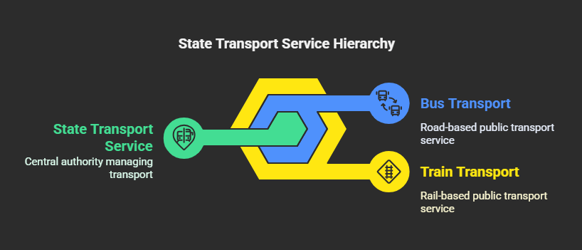
Think of your local transit agency as a dependency container. You just want to get from Point A to Point B, right? If the train’s out of commission, the agency swaps in a replacement bus, no problem. You don’t really care how they get you there, just that you arrive.

Disclaimer: Analogies are helpful, but they don’t always align perfectly. Let’s explore how this real-world scenario, despite its limitations, mirrors the powerful concept of dependency injection in software engineering.

Why

Software maintenance dominates engineering time, far outweighing new development. Simplicity is the key to manageable maintenance. Just as mechanics prefer Toyota’s straightforward engines to BMW’s complexity, engineers work more effectively with clean, well-structured code.

Dependency Injection makes software more flexible because components can be easily swapped out (like replacing that engine with a different one). It also makes testing easier since you can substitute real components with test versions. And maintenance becomes simpler because changes to one component don’t necessarily require changes to others.

How

Let’s get straight to the code

// Interface that defines our transit service contract
public interface ITransitService
{
    string GetTransitInfo();
}

// Implementation for train transit
public class TrainTransitService : ITransitService
{
    public string GetTransitInfo()
    {
        return "Train departing from platform 3 at 14:30";
    }
}

// Implementation for bus transit
public class BusTransitService : ITransitService
{
    public string GetTransitInfo()
    {
        return "Bus departing from bay 7 at 15:15";
    }
}

[ApiController]
[Route("api/[controller]")]
public class TransportController : ControllerBase
{
    private readonly ITransitService _transitService;

    // Constructor injection - the dependency is injected here
    public TransportController(ITransitService transitService)
    {
        _transitService = transitService;
    }

    [HttpGet]
    public IActionResult Get()
    {
        return Ok(_transitService.GetTransitInfo());
    }
}

public class Program
{
    public static void Main(string[] args)
    {
        var builder = WebApplication.CreateBuilder(args);

        builder.Services.AddControllers();
        
        // Register the service implementation to use
        // Change this line to use TrainTransitService instead if 
// needed or this can be controller 
// via some external config/parameter which swaps this dynamically
        builder.Services.AddScoped<ITransitService, BusTransitService>();

        var app = builder.Build();

        app.MapControllers();

        app.Run();
    }
}

Keep it clean, keep it maintainable, and you’ll thank yourself later when you’re not spending your weekends debugging spaghetti code instead of enjoying actual spaghetti!

Now, go fix some bugs!

Re-ranking in Vector search

Analogy to define the problem

Imagine a child has a big box of Lego bricks of various colors. They’re asked to build a tower, but with a special rule: the bricks that are most similar to the color red should be placed at the top, and the bricks that are least similar to red should be at the bottom. Now, let’s say you introduce a condition to complete it in the shortest possible time.

In the shortest possible time, there is a chance they may make mistakes and overlook a few things due to the emphasis on speed.

Analogies are fun, but don’t try to make them too perfect – they all break down eventually!

How does this problem apply to vector search

Approximation: Many use approximate nearest neighbor (ANN) techniques for speed, which means they don’t always find the absolute closest vectors, leading to slightly inaccurate rankings.

Vector Representation: The quality of the vector embeddings matters. If the vectors don’t accurately capture the semantic meaning of the data, similarity scores will be misleading.

Distance Metric: The chosen distance metric (e.g., cosine similarity, Euclidean distance) may not perfectly align with the user’s perception of relevance.

Data Distribution: Vector spaces can be high dimensional and sparse, causing the “curse of dimensionality” where distance becomes less meaningful.

What exactly happens in re-ranking

Re-ranking Model

  • The initial search results, along with the query vector, are processed by an advanced model to refine relevance scoring.
  • Typically, this model is transformer-based (e.g., BERT) and trained to capture semantic similarity.
  • It evaluates each document in relation to the query and may also consider contextual relationships among retrieved documents.
  • The model assigns a relevance score to each document, reflecting its alignment with the query.

Re-ordering

  • The retrieved results are re-ranked based on the relevance scores from the re-ranking model.
  • Documents with the highest scores are prioritized at the top of the results list for improved accuracy.

Example Code

import numpy as np
from sklearn.neighbors import NearestNeighbors
from sentence_transformers import SentenceTransformer

# 1. Define sample data
documents = [
    "Machine learning is a subfield of artificial intelligence",
    "Neural networks are used in deep learning applications",
    "Natural language processing deals with text data",
    "Computer vision focuses on image recognition",
    "Reinforcement learning uses rewards to train agents"
]

# 2. Create vector embeddings for documents
encoder = SentenceTransformer('all-MiniLM-L6-v2')
document_embeddings = encoder.encode(documents)

# 3. Build ANN index
ann_index = NearestNeighbors(n_neighbors=3, algorithm='ball_tree')
ann_index.fit(document_embeddings)

# 4. Define user query and convert to embedding
query = "How do AI systems understand language?"
query_embedding = encoder.encode([query])[0].reshape(1, -1)

# 5. Initial Retrieval: Get approximate nearest neighbors
distances, indices = ann_index.kneighbors(query_embedding)
initial_results = [(i, documents[i], distances[0][idx]) for idx, i in enumerate(indices[0])]

print("Initial ANN Results:")
for idx, doc, dist in initial_results:
    print(f"Doc {idx}: {doc} (Distance: {dist:.4f})")

# 6. Re-ranking with a more sophisticated model (simulated here)
def rerank_model(query, candidates):
    # In a real system, this would be a transformer model like BERT
    # Here we simulate with a simple relevance calculation
    relevance_scores = []
    for _, doc, _ in candidates:
        # Count relevant keywords as a simple simulation
        keywords = ["language", "text", "natural", "processing"]
        score = sum(keyword in doc.lower() for keyword in keywords)
        # Add a baseline score
        score += 0.5
        relevance_scores.append(score)
    return relevance_scores

# 7. Apply re-ranking
relevance_scores = rerank_model(query, initial_results)

# 8. Re-order results based on new relevance scores
reranked_results = [(initial_results[i][0], initial_results[i][1], score) 
                    for i, score in enumerate(relevance_scores)]
reranked_results.sort(key=lambda x: x[2], reverse=True)

print("\nRe-ranked Results:")
for idx, doc, score in reranked_results:
    print(f"Doc {idx}: {doc} (Relevance Score: {score:.4f})")

When Re-Ranking Offers Limited Value

Poor initial results: If the first search is bad, re-ranking can’t fix it.

Uniform relevance: If everything is equally relevant/irrelevant, re-ranking is pointless.

Computational cost: Re-ranking is slow, impacting real-time use.

Relevance mismatch: The model’s “relevance” differs from the user’s.

Ambiguous queries: Re-ranking struggles with unclear requests.

Data bias: Biased training leads to biased results.

This serves as a reference to clarify my understanding of the problem, explore a potential solution, and outline its limitations.

Now, go fix some bugs! 🚀

Augmenting part of RAG

augment
verb
/ɔːɡˈmɛnt/

make (something) greater by adding to it.

What

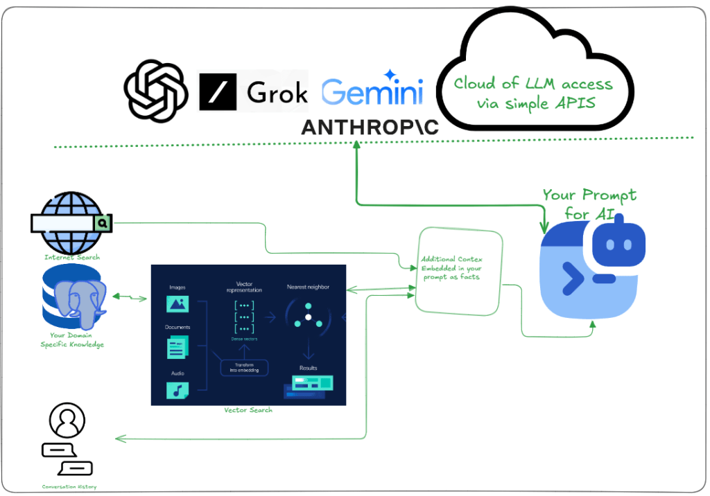
Since “augmenting” implies enhancing or expanding something, it naturally suggests that the LLM — already valuable on its own — serves as the foundation for this improvement. By feeding it additional context, its responses become more accurate, relevant, and informed.

Why

  • Outdated Knowledge: Training data is static.
  • Domain Limits: Lack specialized expertise.
  • Hallucinations: Generate false information.
  • Context Gaps: Limited memory for long interactions.
  • Real-time Needs: Cannot access live data.

How

  • Outdated Knowledge: Implement asynchronous document updates and vector embedding refreshes to maintain current information in the external knowledge base.
  • Domain Limits: Curate domain-specific knowledge bases and employ context-aware fusion mechanisms for tailored information integration.
  • Hallucinations: Utilize relevancy search with vector representations to retrieve and augment LLM prompts with factual, authoritative information.
  • Context Gaps: Apply efficient document retrieval strategies and context management techniques, such as TF-IDF or BM25, to handle large context sizes within model token limits.
  • Real-time Needs: Incorporate dynamic information retrieval components that access up-to-date external data sources before LLM generation

This is by no means a comprehensive guide — rather, it’s a straightforward way of documenting my current understanding. For each of these topics, there are countless resources available to explore in greater depth. Hope this gives your learning a fun boost!

Now, go fix some bugs!

Vector Search, R of the RAG

Photo by David McBee on Pexels.com

What

A vector is a quantity that has both magnitude (or length) and direction. A vector might represent the features of an image or a piece of text. In this context, the numbers within the vector represent values of those features.

Why

Imagine you’re searching for a car with a red color. In a traditional keyword search, you’d need the car’s description to explicitly mention “red color” to get a match. But car companies rarely keep it that simple — instead, they use creative names like “Cherry Bomb Tintcoat” or “Rosso Corsa”. A keyword search would struggle to connect your “red color” query with these fancy names. However, with vector search, the system understands the underlying meaning and context, so even abstract color names show up — ranked by a relevance score that reflects how closely your query aligns with the results.

How

Vector search, powered by embeddings, allows systems to understand the meaning of words and phrases. Embeddings convert text into numerical vectors that represent their semantic relationships.

Example

from sklearn.metrics.pairwise import cosine_similarity
import numpy as np
from sentence_transformers import SentenceTransformer

# Initialize a pre-trained sentence transformer model
model = SentenceTransformer('all-MiniLM-L6-v2')

# Sample car color names (like a car database)
car_colors = [
    "Cherry Bomb Tintcoat",
    "Rosso Corsa",
    "Soul Red Crystal Metallic",
    "Firecracker Red",
    "Carmine Red",
    "Race Red",
    "Ruby Flare Pearl"
]

# Convert car color names to vectors (embeddings)
color_embeddings = model.encode(car_colors)

# User query
user_query = "I want a car with red color"

# Convert user query to vector
query_embedding = model.encode([user_query])

# Calculate cosine similarity between query and car color names
similarities = cosine_similarity(query_embedding, color_embeddings)[0]

# Rank results by similarity score
ranked_results = sorted(zip(car_colors, similarities), key=lambda x: x[1], reverse=True)

# Display top results
print("Top matches for your query:\n")
for car_color, score in ranked_results[:3]:
    print(f"{car_color} (Relevance Score: {score:.2f})")

This approach offers a more effective way to retrieve relevant contextual information or facts based on a user’s query or question. In the context of Retrieval-Augmented Generation (RAG), this information enhances the model’s responses by grounding them in accurate, relevant data. I’ll dive deeper into how this works in my next post.

Now, go fix some bugs! 🚀
Syntactic sugar of async await in JavaScript

Syntactic sugar header image

Most advances in modern programming languages, are striving towards making code more human readable. Some people call these features syntactic sugar, because often it doesn’t really change the way the runtime internally handles it.

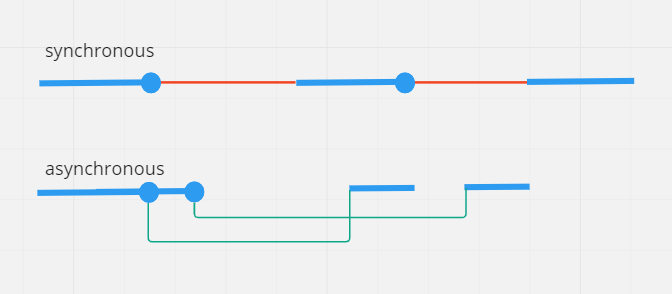
One such feature in JavaScript is async await. Lets first look at the simple diagram, comparing synchronous vs asynchronous calls. Courtesy of Marijn Haverbeke’s amazing book Eloquent JavaScript.

In below diagram, thick blue line is the program running usually and the thin red line represents time spent waiting. As you can see, with asynchronous mode, there is no time spent waiting. hence the primary thread is free to do other things, remains ready for interactivity. It picks up the processing on a future callback e.g. an API call returning a response.

Diagram explaining difference between synchronous and asynchronous timelines

Analogy, lets say you drop your friend to do some shopping. He is going to call you when he is done. If you wait outside doing nothing, waiting for his call, that is stupid(synchronous). If you go do some of your other chores, and when he calls, you go back to pick him up, that is smart(asynchronous).


So, asynchronous is good, how to do it in JS, two prominent ways are promises and async await

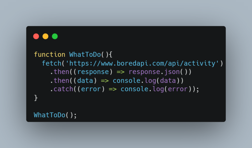
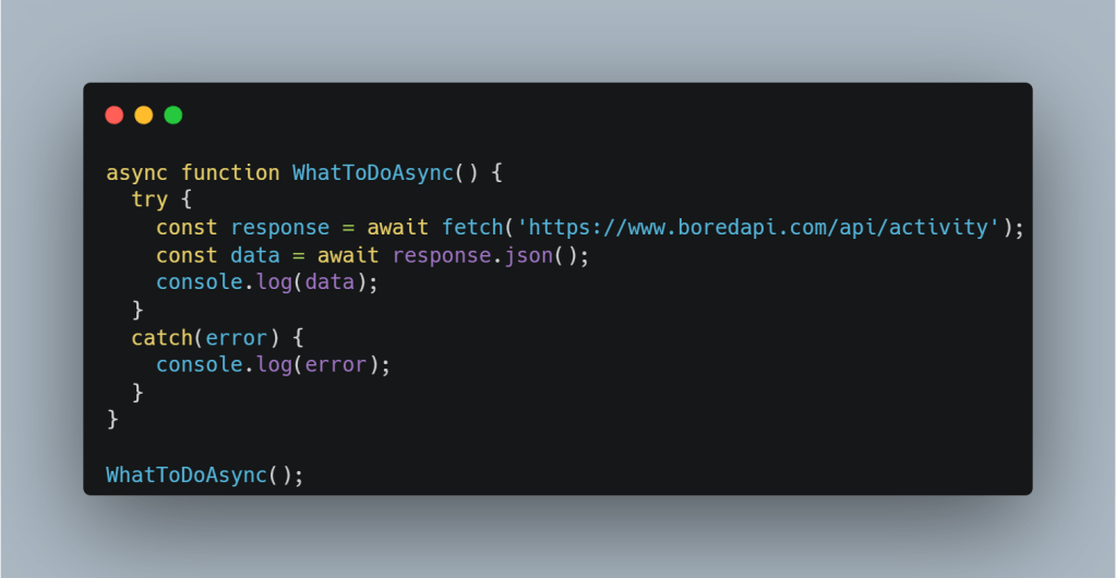
Enough english and images, lets see the code. Where the same API call is done both ways. API returns a response and then its converted to JSON, both return a promise.

async await code sample

In case you are wondering that’s a real API, and you can see these examples in action at this jsfiddle

You might say, its not making any difference to number of lines of code, but the point is readability. In this contrived example may not seem much but in many real world applications, promises are chained at much deeper level causing readability hell.

Now, go fix some bugs!

The point of Svelte stores

Why

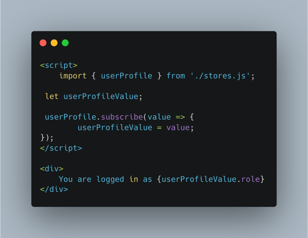
In single-page applications, different pages are constructed using components. Often you need to share some data across them. Also, after the initial server render further interactions happen on the client-side, so, you need some way to store the initial state you got from the server.

What

Many frameworks have their respective recommended way of managing the state. Angular has Rxjs, React with Redux, and Svelte has Svelte-stores

How

Instead of how these state libraries work internally, let’s look at how these are used in an app, specifically Svelte.

Diagram

An image always makes more sense before we look at the code 

Code

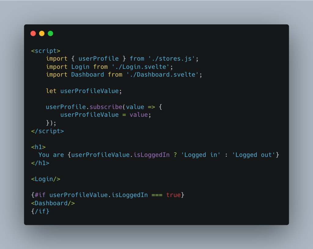
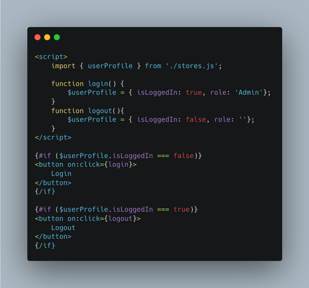
Working Sample Code hosted online at REPL

App.svelte

Login.svelte

Dashboard.svelte

store.js

Now, go fix some bugs!

Using emojis to understand JS Spread and Destructuring

This is in a quest to explain things to a five-year-old(myself). And what better way than to have some pictures than text.

Spread (…)

Prefixing an array, string, or an object with spread(...) when calling a function or as part of an assignment will expand the array elements, in case of object into key-value pairs.

Array example

Object example

Destructuring

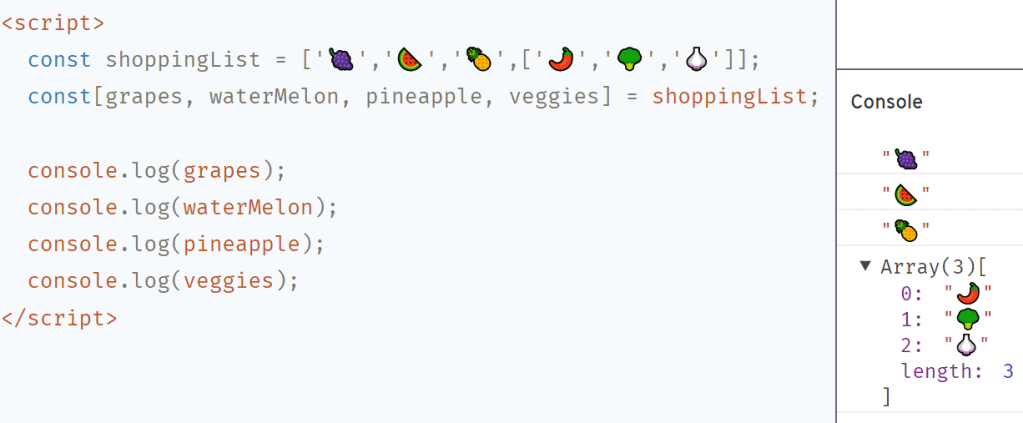
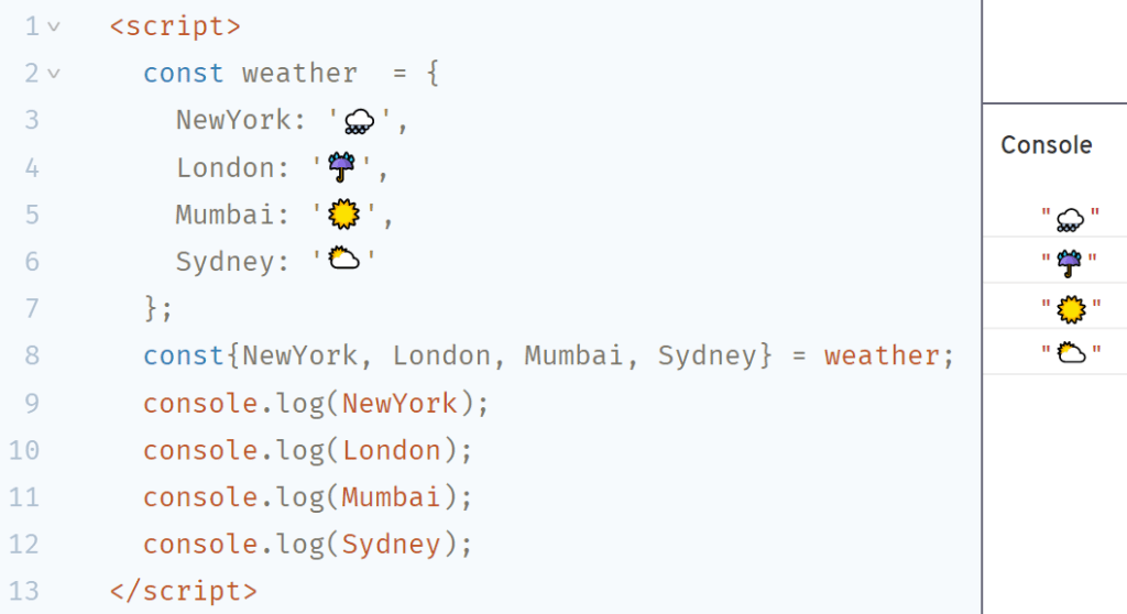
Destructuring isn’t really related or similar to spread but just an easy way of extracting values from arrays and objects into variables.

Array example

Object example

There are so many different ways you can use destructuring, but the information is better retained if it is gathered in steps. I hope this is a simpler start for getting your head around these concepts.

Now, go fix some bugs!